
Contents:
Data powers machine learning solutions. Quality datasets enable training models with the needed detection and classification accuracy, though sometimes the accumulation of sufficient training data that should be fed into the model is a complex challenge. For instance, to create data-intensive apps, human annotators are required to label a huge number of samples which results in complexity of management and high costs for businesses. In addition to that, there is a difficulty of data acquisition related to safety regulations, privacy, or ethical concerns.
When we have a limited dataset including only a finite number of samples per class, few-shot learning may be useful. This model training approach helps make use of small datasets and achieve acceptable levels of accuracy even when the data is fairly scarce.
In this article, I will explain what few-shot learning is, how it works under the hood, and share with you the results of research on how to get optimum results from a few-shot learning model using a relatively simple approach for image classification tasks.
Before moving to technologies and principles under the hood of Few-Shot learning, let’s have some fun.
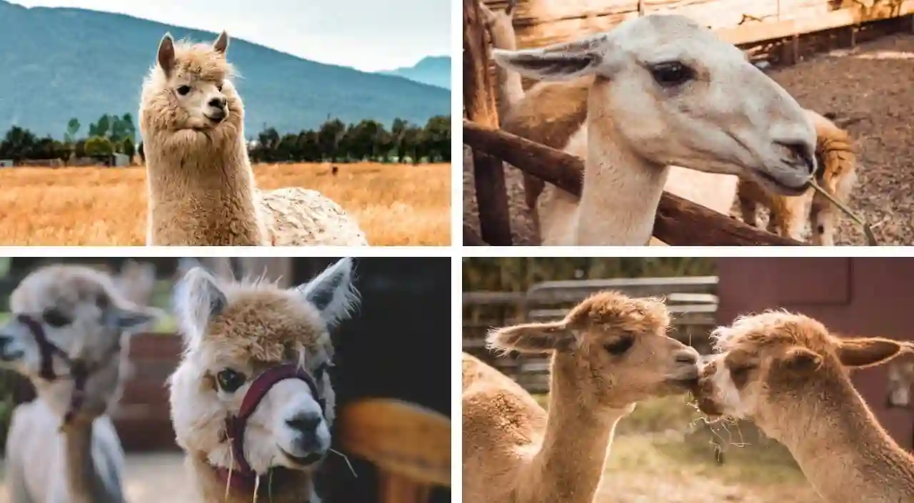
The left side of the image depicts an alpaca, and the right side is a representation of a llama. These animals are similar, although there are differences. The crucial distinctions are that llamas are bigger and heavier than alpacas; also, they have long snouts, while alpaca’s snouts are flattened. The most readily distinguishable difference is that llamas have long rounded ears that resemble bananas, while alpaca’s ears are short and pretty.
You’ve learned to distinguish the two animals from the Camelidae family. Taking into account the difference in ears, try to guess what animal is depicted in the query image below.

You’ve probably found out that it’s a llama. Four samples are enough for humans to distinguish one animal from another, even though these animals look similar. But will a computer be able to deal with such a task? Can the machine make the appropriate prediction if the class consists of two samples?
The task is more complicated than normal object classification because a lack of samples makes it impossible to train a deep neural network from scratch. That’s where few-shot learning comes in.
What is Few-Shot Learning?
The starting point of machine learning app development is a dataset, and the more data, the better result. Through obtaining a big amount of data, the model becomes more accurate in predictions. However, in the case of few-shot learning (FSL), we require almost the same accuracy with less data. This approach eliminates high model training costs that are needed to collect and label data. Also, by the application of FSL, we obtain low dimensionality in the data and cut the computational costs.
Note that FSL can be mentioned as low-shot learning (LSL) and in some sources this constitutes ML problems where the volume of the training dataset is limited.
- FSL or LSL problems can be related to business challenges. It could be object recognition, image classification, character recognition, NLP, or other tasks. The machines are required to perform them and navigate the rare cases through the application of FSL techniques with a small amount of training data. A notable example of FSL is connected with the robotics field. In this example, robots learn how to move and navigate after getting acquainted with a few demonstrations.
- If we apply only one demonstration to train the robot, it would be a one-shot ML problem. In individual cases, when not all classes are labeled in the training, we face zero training samples for the particular categories and a zero-shot ML problem.
Approaches of Few-shot Learning
To tackle few-shot and one-shot machine learning problems, we can apply one of two approaches.
1. Data-level approach
If there is a lack of data to fit the algorithm and to avoid overfitting or underfitting of the model, then additional data is supposed to be added. This algorithm lies at the core of the data-level approach. The external sources of various data contribute to its successful implementation. For instance, solving the image classification task without sufficient labeled elements for different categories requires a classifier. To build a classifier, we may apply the external data sources with similar images, even though these images are unlabeled and integrated in a semi-supervised manner.
To complement the approach, besides external data sources, we can use the technique that attempts to produce novel data samples from the same distribution as the training data. For example, the random noise added to the original images results in generating new data.
Alternatively, new image samples can be synthesized using the generative adversarial networks (GANs) technology. For example, with this technology, new images are produced from different perspectives if there are enough examples available in the training set.

2. Parameter-level approach
The parameter-level approach involves meta-learning — the technique that teaches the model to understand which features are crucial to perform machine learning tasks. This can be achieved by developing a strategy for controlling how the model’s parameter space is exploited.
Limiting the parameter space helps to solve challenges related to overfitting. The basic algorithm generalizes a certain amount of training samples. Another method for enhancing the algorithm is to direct it to the extensive parameter space.
The main task is to teach the algorithm to choose the most optimal path in the parameter space and give targeted predictions. In some sources, this technique is mentioned as meta-learning.
Meta-learning employs a teacher model and a student model. The teacher model sorts out the encapsulation of the parameter space. The student model should become proficient in how to classify the training examples. Output obtained from the teacher model serves as a base for the student’s model training.
Applications of Few-shot Learning
Few-shot learning forms the basic algorithm for applications in the most popular fields (Fig. 1), namely:
- Computer Vision
- Natural Language Processing
- Robotics
- Audio processing
- Healthcare
- IoT
In computer vision, FSL performs the tasks of object and character recognition, image and video classification, scene location, etc. The NLP area benefits from the algorithm by applying it to translation, text classification, sentiment analysis, and even criminal charge prediction. A typical case provides for character generation as machines parse and create handwritten characters after a short training on a few examples. Other use cases include object tracking, gesture recognition, image captioning, and visual question answering.
Few-shot learning assists in training robots to imitate movements and navigate. In audio processing, FSL is capable of creating models that clone voice and convert it across various languages and users.
A remarkable example of a few-shot learning application is drug discovery. In this case, the model is being trained to research new molecules and detect useful ones that can be added in new drugs. New molecules that haven’t gone through clinical trials can be toxic or low active, so it’s crucial to train the model using a small number of samples.
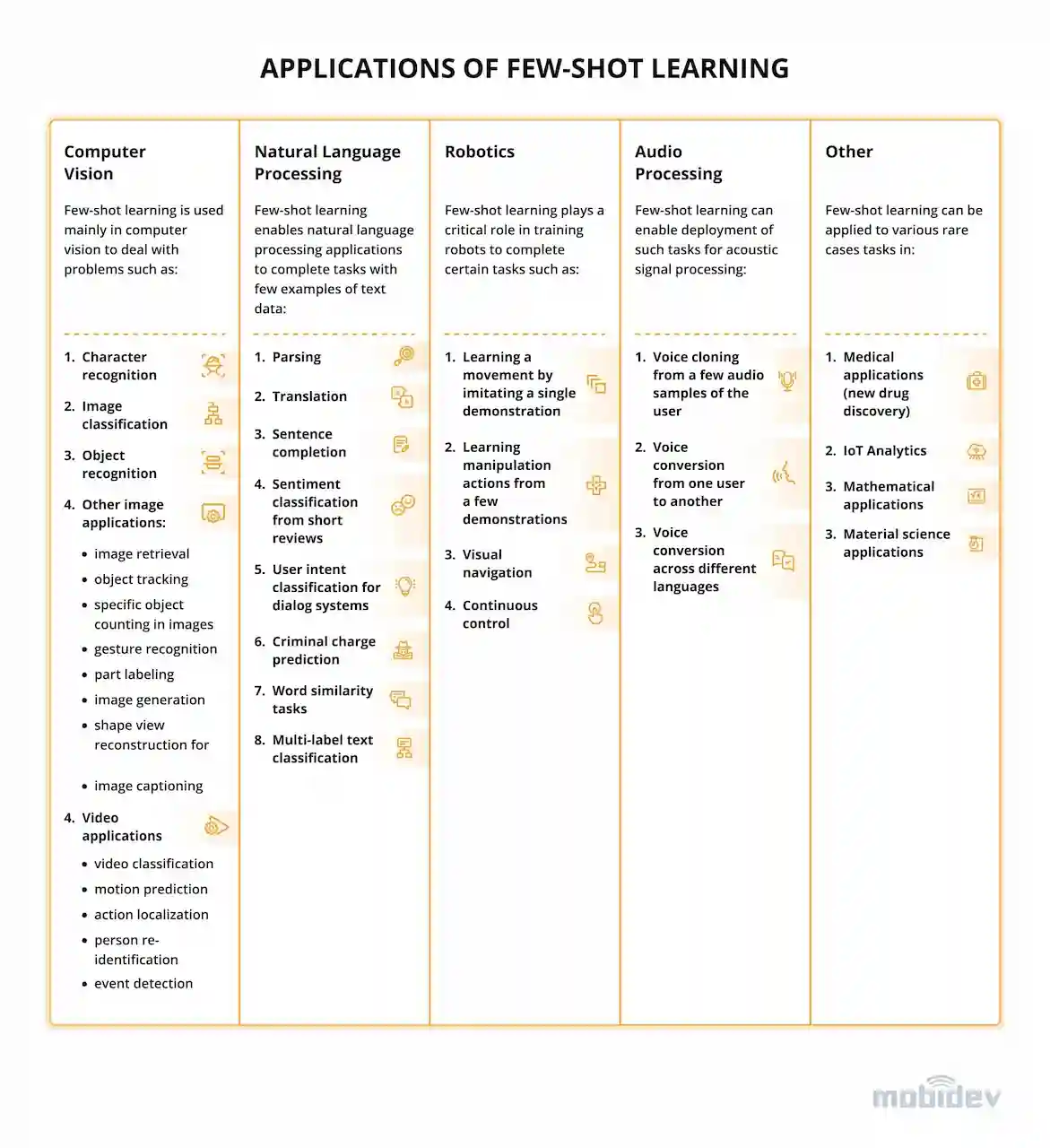
Figure 1. Few-shot learning applications
Let’s take a deeper dive into how few-shot learning works and overview the results of MobiDev’s research.
Research: Few-shot Learning For Image Classification
We selected a problem of image classification. A model has to determine the category the image belongs to for the identification of a denomination of a coin. This could be used to quickly count the total sum of coins lying on a table by splitting the larger image into smaller ones containing individual coins and classifying each small image.
Data sets
First of all, we needed some few-shot learning data to experiment with. For this purpose, we collected a dataset of euro coin images from public sources with 8 classes according to the number of coin denominations (Fig. 2).
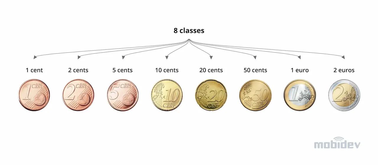
Figure 2. Image classes with examples
The data was split into 3 subsets – support (train), query (val), and test set (statistics on the datasets can be seen in the Fig. 3). Support and query datasets were selected to be from one distribution whereas the test dataset was purposefully chosen to come from a different one — images in the test are over/underexposed, tilted, show coins with unusual colors, contain blur, etc.
This data preparation was done to simulate the production setting where the model is often trained and validated on good quality data from open datasets / internet scraping, whereas the data from the real operation conditions is usually different: users can capture images with different devices, have poor lighting conditions, and so on. A robust CV solution should be able to tackle these problems to a certain extent, and our goal is to figure out how this will work out for a few-shot learning approach which assumes we do not have much data to begin with.
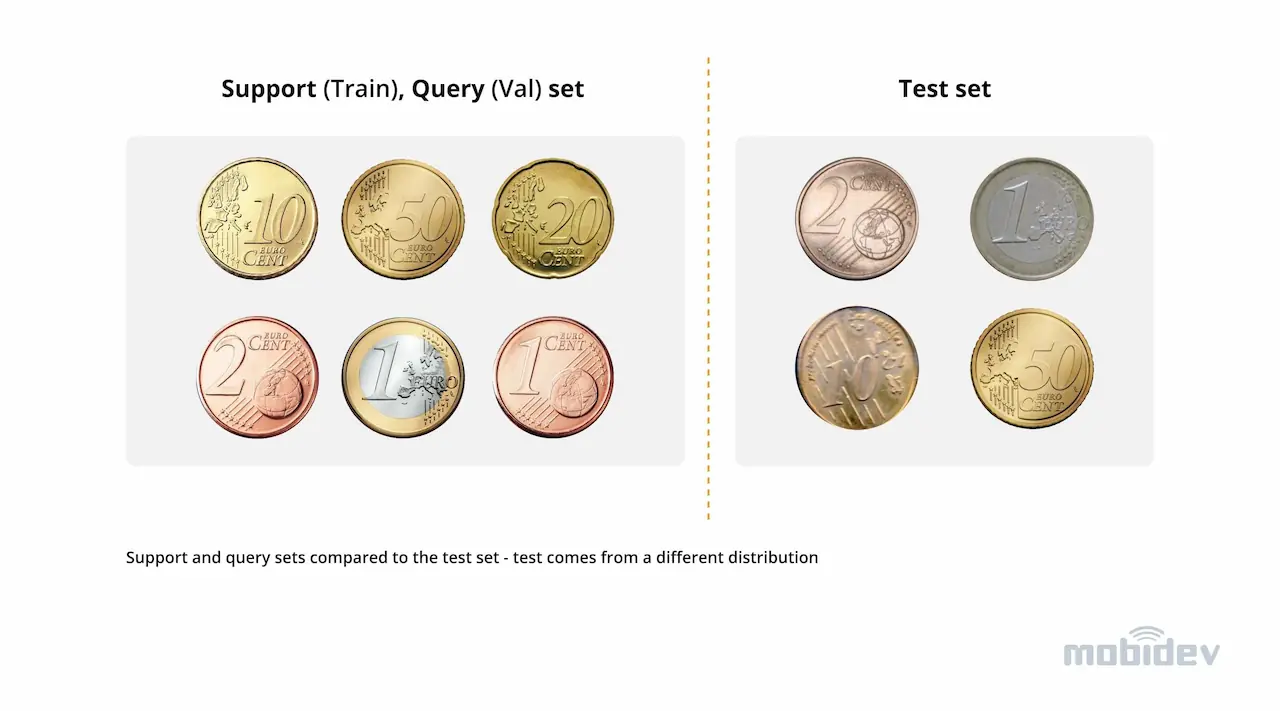
Figure 3. Support and query sets compared to the test set – test comes from a different distribution
Finally, the statistics on the number of available data samples can be seen in Fig. 4. We managed to collect 121 data samples, ~15 images per coin denomination. The support set is balanced, each class has an equal amount of samples with up to 4 images per class for few shot training, while the query and test sets are slightly imbalanced and contain approx. 7 and 4 images per class respectively. The number of samples per set: support — 32, query — 57, test — 31.
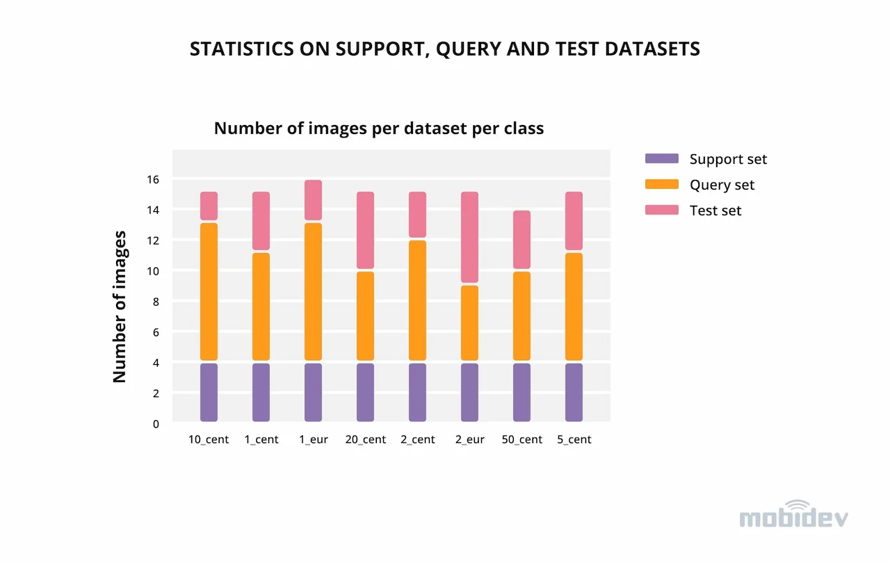
Figure 4. Statistics on support, query, and test datasets
Selected approach
In the selected approach, we use a pre-trained Convolutional Neural Network (CNN) as an encoder to obtain compressed image representations. The model is able to produce meaningful image representations that reflect the content of the images since it has seen a large dataset and was pre-trained on ImageNet prior to few-shot learning. These image representations can then be used in few-shot learning and classification.
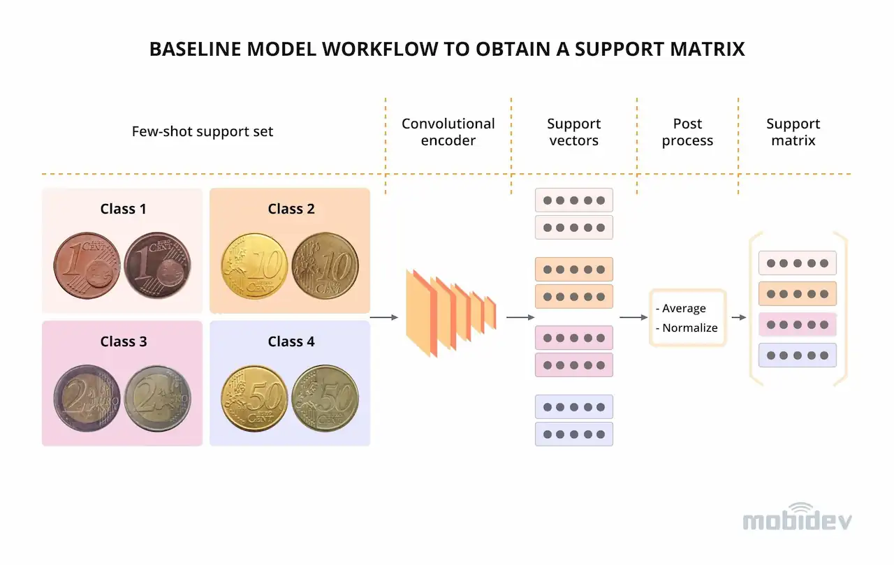
Figure 5. Baseline model workflow to obtain a support matrix
Multiple steps that can be taken to improve the performance of a few-shot learning algorithm:
- Baseline (Fig. 5)
- Fine-tuning
- Fine-tuning + Entropy Regularization
- Adam optimizer
To learn more about each step, download the full PDF version of the research below.
The Experiment Results
With the selected model configuration, we ran several experiments on the collected data. First of all, we used a baseline model without any fine-tuning or additional regularization. Even in this default setting the results were surprisingly decent as illustrated in Tab. 1: 0.66 / 0.62 weighted F1 score for query / test sets. We chose a weighted F1 metric as it takes into account imbalance in class sizes as well as combining both precision and recall scores.
At this stage, we experimented with the size of the support set. As expected, larger support set results in better query and test performance, although the benefits of using more samples reduce as the train set size increases (Fig. 6).
Interestingly, with small support set sizes (1-3) there are random shifts in query vs test set performances (one can improve while the other decreases), however, at support set size 4, there is an improvement for both of the sets.
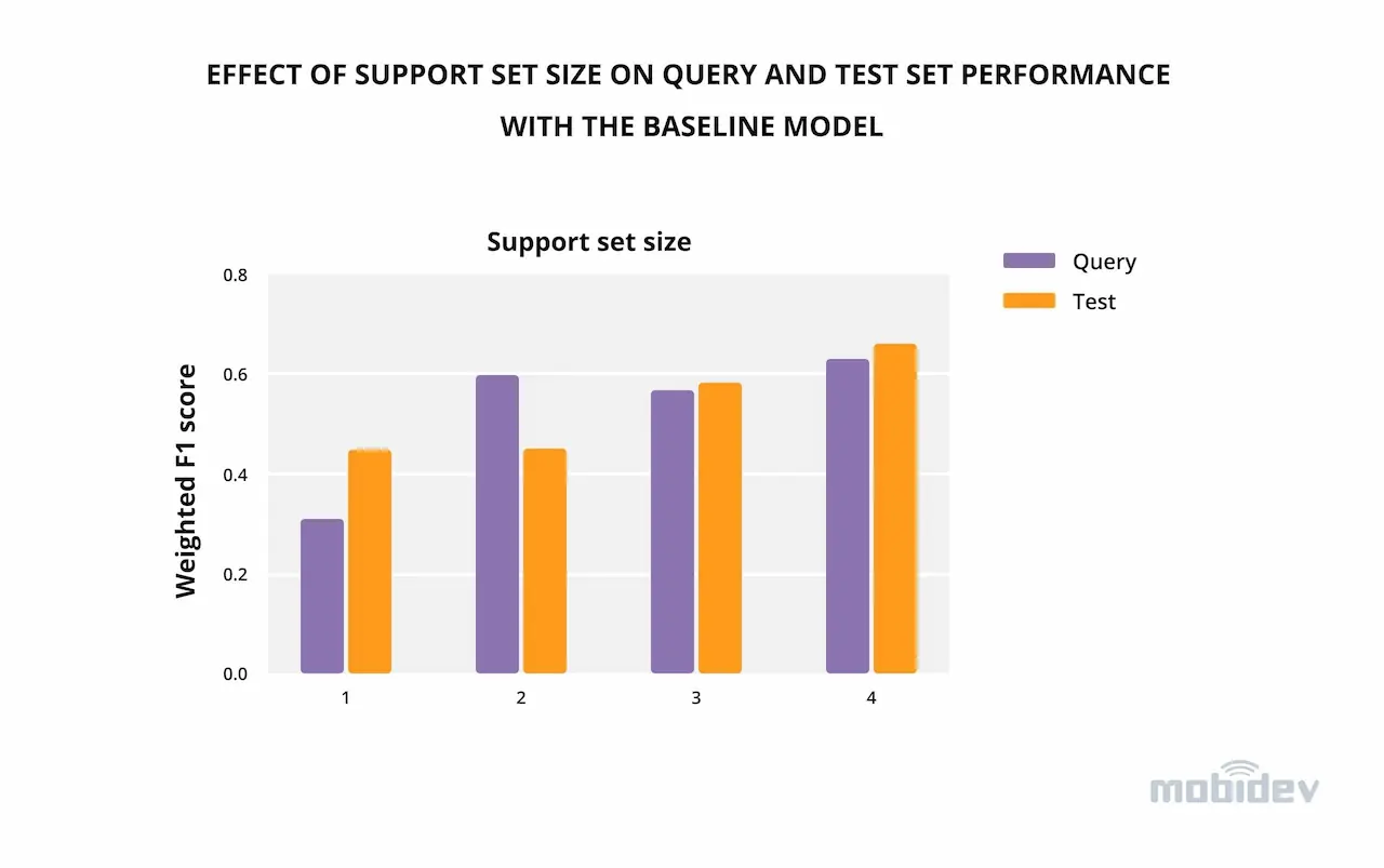
Figure 6. Effect of support set size on query and test set performance with the baseline model
Moving on from the baseline model, fine-tuning with the application of Adam optimizer on mini-batches from the support set improves the scores by 2% for both query and test sets. This result is further enhanced by 1-4 % when adding entropy regularization on the query set into the fine-tuning pipeline.
It is important to point out that accuracy improves alongside the weighted F1 score, meaning that the model performs better not only class-wise but also in relation to the total amount of data. The final accuracy of 0.7 and 0.68 for query and test sets means the model that had only 4 image examples for training could successfully guess the class of the image in 40/57 examples for query and 21/31 examples for test set.
Table 1. Few-shot metrics on val/test datasets
| Run settings | Accuracy | Weighted F1 score | ||
|---|---|---|---|---|
| Query set | Test set | Query set | Test set | |
| Baseline | 0.67 | 0.61 | 0.66 | 0.62 |
| Baseline + fine tuning | 0.68 | 0.65 | 0.68 | 0.64 |
| Baseline + fine tuning + regularization | 0.7 | 0.68 | 0.69 | 0.69 |
Looking at the confusion matrix on the query set (Fig. 7), we can spot some interesting tendencies. Firstly, the easiest for the model categories to guess were large nominal coins 1 and 2 euro because these coins are made of two parts: inner and outer. Two parts immediately make them distinctive from small nominal coins.
In addition, in 1 euro the inner part is made of grey copper-nickel alloy, while the outer part is composed of golden nickel-brass alloy. In 2 euro coins, the alloys are reversed: copper-nickel for the outer part and nickel-brass for the inner part. This peculiarity makes it easier to differentiate one coin from another.
Two difficult to figure out combinations were 20 vs 50 cents and 5 vs 2 cents, as the model often confused these coins between each other. This was because of little difference between these categories: the color, the shape of the coins, and even the textual inscriptions are the same. The only distinction is the actual denomination inscription of the coin. Since the model was not specifically trained on coins, it does not know which areas of the coins it should be paying the most attention to and therefore can undervalue the importance of denominal value inscriptions.
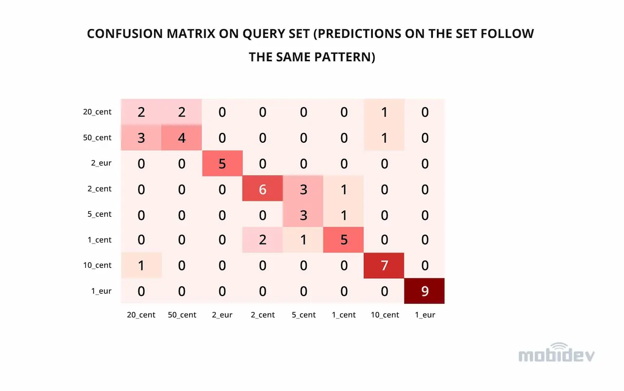
Figure 7. Confusion matrix on query set (predictions on the set follow the same pattern)
Wrapping Up
In a demanding world of practical Machine Learning, there is always a balance between the accuracy of the developed solutions and the amount of work and data the solution requires. Sometimes, it is preferable to quickly create a solution that meets only minimum accuracy requirements, deploy it in production, and iterate from there. In this scenario, the approach described in this article could work well.
We found out that for a problem of a few-shot classification of coins by image, it is possible to reach ~70% accuracy given as few as 4 image examples per coin denomination.
The problem is quite difficult for a model pre-trained on a broad set of data (ImageNet dataset) as the model does not know which specific part of a coin it should focus on to make an accurate prediction, and we expect the accuracy could be even higher given a problem where distinctive features would be more evenly distributed across the image (e.g. fruit type and quality classification).


